Notes on Dimensionality Reduction
It is often possible to compress datasets into lower dimensions while retaining much of their original useful information. This type of compression is particularly beneficial for high-dimensional data, where reducing dimensionality can improve computational efficiency and model performance. One common approach to dimensionality reduction is linear projection, like principal component analysis.
What is the Curse of Dimensionality?
As the number of dimensions in a data set increases, training a model with high predictive power becomes increasingly difficult. The intuition behind this phenomenon is that higher-dimensional spaces become more sparse, meaning data points are naturally farther apart. This sparsity poses a problem because, probabilistically, any new data point your model encounters is likely to be far from the existing training data. Consequently, models trained on high-dimensional data can suffer from poor generalization.
High-dimensional data leads to increased computational complexity. More dimensions require more computation, which results in longer training times and higher resource consumption.
Principal Component Analysis
One of the most widely used dimensionality reduction techniques is Principal Component Analysis (PCA). At a high level, PCA identifies the hyperplane that is closest to the data and projects the data onto it.
How is this hyperplane chosen? We can illustrate this concept by considering a two-dimensional subspace with four unit vectors plotted along with some sample data.
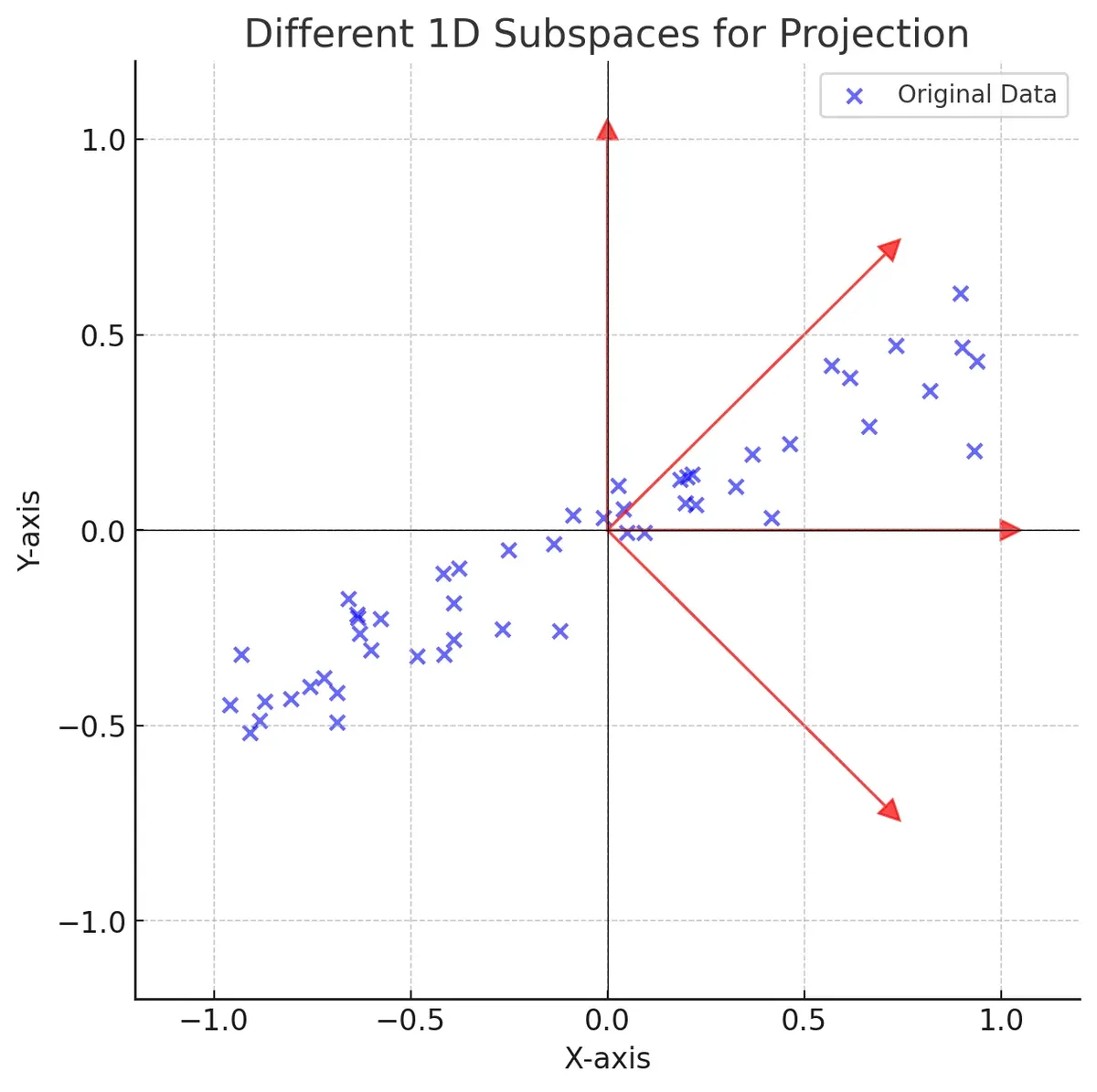
When we perform a linear projection of the data onto each unit vector, we obtain one-dimensional representations of the dataset.
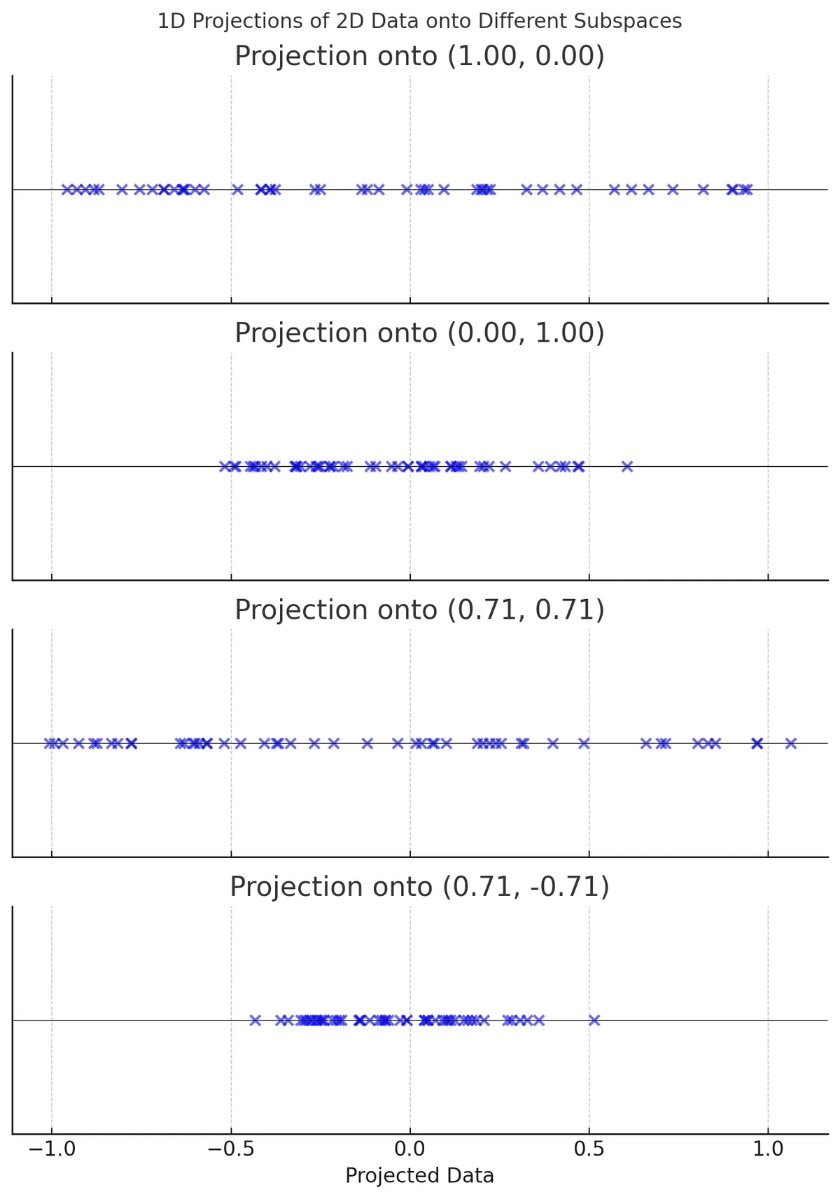
The next question is: Which unit vector provides the best hyperplane for projection?
We should select the one that captures the most variance, as it minimizes the loss of information. Mathematically, this means choosing the hyperplane that minimizes the mean squared distance between the original dataset and its projection onto that axis.
The Explained Variance Ratio
The explained variance ratio quantifies how much of the total variance in the dataset is captured by each principal component. This metric helps determine the effectiveness of dimensionality reduction. The explained variance ratio of a principal component is equal to the ratio of a component's eigenvalue to the sum of the eigenvalues of all the principal components.
A generally useful rule of thumb is to reduce the number of dimensions while preserving 90-95% of the total variance of the dataset. This ensures that most of the essential information is retained.
Random Projection
Random Projection (RP) is another dimensionality reduction technique that maps high-dimensional data onto a lower-dimensional space using a random linear projection. Unlike PCA, which finds the optimal hyperplane that maximizes variance preservation, RP selects a random hyperplane and projects onto it.
The core idea underpinning RP is the Johnson-Lindenstrauss Lemma, which states that if you project points from a higher-dimensional space, , to a lower dimensional space, , then the distances between points are approximately preserved. In order for RP to work, has to be chosen properly. The following relation can be used to compute :
In the above relation, , is the distortion parameter which controls how much the distances are preserved in the lower-dimensional space.
Conclusion
Reducing dimensionality can be a useful tool to compress a dataset into its most useful information. This makes it easier to train a model on the data. Techniques like PCA and RP can help improve the efficiency of training while preserving the variance in a dataset.